Processing the time-lapse images

Extracting timestamps from a time lapse video

This post will outline the workflow I created to extract time-stamps from a time-lapse video. The time-lapse camera I have been using has very little flexibility in setting the the play back frame rate of the stored video. In addition, I wanted to remove all the night time images except for one frame, so the transition from one day to another is obvious.

The way I have approached this was to;

  1. Use imagemagick to extract all of the frames as jpeg images from the time-lapse video.
  2. Extract the date characters from each image and use an artificial neural network to classify each character to determine the time of each image.
  3. Use a second neural network to determine if the image was taken at night (dark) or during the day (light).
  4. Use ffmpeg to stitch the images back together at my desired frame rate.

Load and examining the training dataset

The first step requires the use of a training set of all the characters to build train a neural network model. Therefore the first set of images must be loaded into R (I manually cropped them before this).

# Load the jpeg library
library(jpeg)
# Load the training set - rounding each pixel off to 0 or 1.
number_zero <- round(
  readJPEG(
    "_Rmd/training_set/number_wang/number_zero.jpeg"
    )
  )
number_one <- round(
  readJPEG(
    "_Rmd/training_set/number_wang/number_one.jpeg"
    )
  )
number_two <- round(
  readJPEG(
    "_Rmd/training_set/number_wang/number_two.jpeg"
    )
  )
number_three <- round(
  readJPEG(
    "_Rmd/training_set/number_wang/number_three.jpeg"
    )
  )
number_four <- round(
  readJPEG(
    "_Rmd/training_set/number_wang/number_four.jpeg"
    )
  )
number_five <- round(
  readJPEG(
    "_Rmd/training_set/number_wang/number_five.jpeg"
    )
  )
number_six <- round(
  readJPEG(
    "_Rmd/training_set/number_wang/number_six.jpeg"
    )
  )
number_seven <- round(
  readJPEG(
    "_Rmd/training_set/number_wang/number_seven.jpeg"
    )
  )
number_eight <- round(readJPEG(
  "_Rmd/training_set/number_wang/number_eight.jpeg"
  )
  )
number_nine <- round(
  readJPEG(
    "_Rmd/training_set/number_wang/number_nine.jpeg"
    )
  )
slash  <- round(
  readJPEG(
    "_Rmd/training_set/number_wang/slash.jpeg"
    )
  )
dots  <- round(
  readJPEG(
    "_Rmd/training_set/number_wang/dots.jpeg"
    )
  )
# Combine all of teh examples into a single matrix
covars <- rbind(
  matrix(dots, nrow=1),
  matrix(slash, nrow=1),
  matrix(number_zero, nrow=1),
  matrix(number_one, nrow=1),
  matrix(number_two, nrow=1),
  matrix(number_three, nrow=1),
  matrix(number_four, nrow=1),
  matrix(number_five, nrow=1),
  matrix(number_six, nrow=1),
  matrix(number_seven, nrow=1),
  matrix(number_eight, nrow=1),
  matrix(number_nine, nrow=1))

Have a look at the training set using ggplot2

# Load ggplot2 and ggthemes
library(ggplot2)
library(ggthemes)
# Re-format the trainset matrix into a ggplot2 friendly data frame
image_df <- data.frame(x=rep(rep(1:14, each=14), 12),
                 y=rep(rep(14:1, 14), 12), 
                 z=matrix(sapply(1:dim(covars)[1], function(x) covars[x,])),
                 character = rep(c(":", "/", 0:9), each = 196))
 
ggplot() + geom_raster(aes(x,y,fill=factor(z)),image_df) + facet_wrap(~character) + 
  theme_few(15) + scale_fill_manual(guide = "none",values = c("black", "white"))
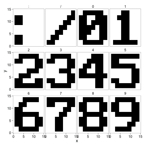
plot of chunk unnamed-chunk-2

Fit the first neural network

The next section will fit a neural network to the training matrix from above. The training set in this case is the covariates for the neural network, where each row of the covariate matrix contains the pixel values for each character and each column of the covariate matrix representing the value of a certain pixel (e.g. (1,1) of each character). In addition the nnet function needs to know which row of the training set represents which character (the y variable).

# Create a vector with the factors of each row in the training set
timestamp_values <- as.factor(c(":", "/",0,1,2,3,4,5,6,7,8,9))
library(nnet)
# Create a matrix with the correct result labeled in the matrix
nums <- class.ind(timestamp_values)
# Fit the model.
set.seed(1750)
mod <- nnet(x=covars, y = nums, 
            size = 4, 
            maxit = 20000, 
            rang = 0.1, 
            decay = 5e-4,
            trace = FALSE)

An example of extracting the time-stamp

This next section will outline how to use the neural network to extract the time-stamp from the original frame of the time lapse images. The original image for this example is:
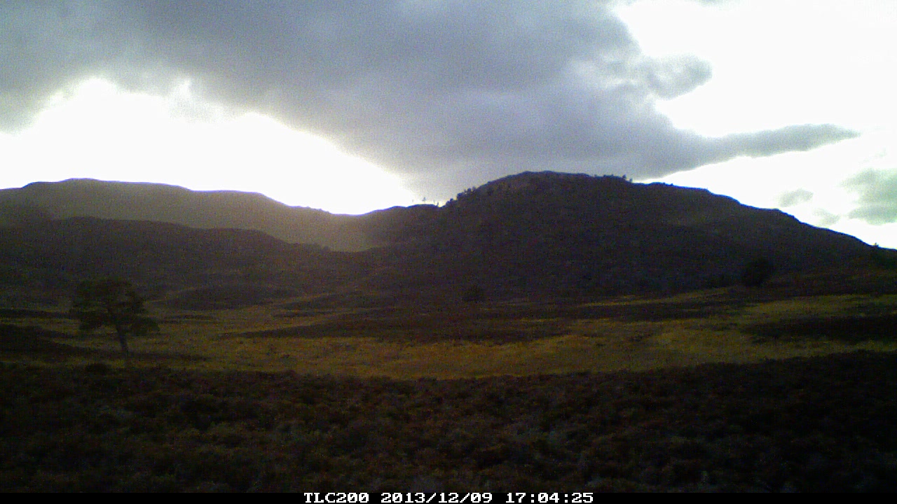
Example image

Firstly, two helper functions are required. The first of these functions uses imagemagick to crop the time-stamp from the bottom of the image and convert it to grey-scale.

# This function creates a black and white image and crops the image 
# to the timestamp (manually).
extract_datestamp <- function(filename){
  system(paste0("convert -negate -type Grayscale -threshold 80% ",
                filename," -gravity South -crop 320x14+53+2 tmp.jpeg" ))
  unknown <- round(readJPEG("tmp.jpeg"))
  unlink("tmp.jpeg")
  return(unknown)
}

The next function finds and extracts the characters from the cropped image above and returns the pixels of each character in a matrix with each row being each individual character. This function will go across the image from left to right. It will look at each column of pixels and determine the start of a character when one or more pixels in the column are white, and the end of that character when all pixels are black.

find_characters <- function(x, ncol, nrow ){
  character_list <- list()
  index <- 1
  i = 1
  while(i < ncol(x)){
    
    if(sum(x[,i])<nrow(x)){
      tmp <- matrix(1, nrow = 1, ncol=ncol*nrow)
      j=1
      while(sum(x[,i])<nrow(x)){
        tmp[j:(j+ncol-1)] <- x[,i]
        j = j+ncol
        i = i+1
      }
      character_list[[index]] <- tmp
      index = index+1
    }
    i = i+1
  }
  
  character_matrix <- do.call("rbind",character_list)
  return(character_matrix)
}

And finally the interesting part extracting the time-stamp from the jpeg image. Here is what image looks like after cropping and converting to grey-scale using imagemagick.

# Get the filename
file_to_test <- list.files("_Rmd/training_set/example")
# Use the helper function to extract the timstamp from the image
unknown <- extract_datestamp(paste0("_Rmd/training_set/example/",file_to_test))
# Format the matrix to create an image with ggplot2
image_df <- data.frame(x=rep(14:1, each=320),
                 y=rep(1:320, 14), 
                 z=matrix(sapply(1:dim(unknown)[1], function(x) unknown[x,])))
# Plot up the timestamp to have a look at it.
ggplot() + geom_raster(aes(y,x,fill=factor(z)),image_df) +
  theme_few(15) + scale_fill_manual(guide = "none",values = c("black", "white"))

plot of chunk unnamed-chunk-6

# Build a matrix of the characeters in the timestamp.
characters <- find_characters(unknown, 14,14)
# Predict each of the characters
predicted_characters <- levels(timestamp_values)[max.col(predict(mod, characters))]

And now the lubridate package can be used to put the characters together and format them as a date object. Did it get it right?

library(lubridate)
date <- ymd_hms(paste(predicted_characters, collapse=""))
date
## [1] "2013-12-09 17:04:25 UTC"

Predicting night or day

The next stage of the image processing is to determine if the image is taken during the day or at night. The easiest solution I could think of to solve this was to shrink the larger image down to a workable size (2% of the original size) and fit a new neural network model to predict if the image is dark or not.

The get_sample function uses imagemagick to rescale and convert the image to grey-scale and load it in to R as a matrix.

# This function shrinks the image, converts it to black and white and loads 
# it in as a matrix.
get_sample <- function(filename){
  system(paste0("convert -negate -resize 2% -type Grayscale ",filename," tmp.jpeg" ))
  large <- readJPEG("tmp.jpeg")
  unlink("tmp.jpeg")
  matrix(large, nrow = 1)
}

Now load in the training set. I have pre-selected several dark and light images to use to train the neural network.

# load the daytime images first.
day_files <- list.files("_Rmd/training_set/day_night/day_examples")
day_examples <- matrix(NA,  length(day_files),364)
for(i in 1:length(day_files)){
  day_examples[i,] <- get_sample(paste0("_Rmd/training_set/day_night/day_examples/",
                                        day_files[i]))
}
# Now load in the night time images
night_files <- list.files("_Rmd/training_set/day_night/night_examples")
night_examples <- matrix(NA,  length(night_files),364)
for(i in 1:length(night_files)){
  night_examples[i,] <- get_sample(paste0("_Rmd/training_set/day_night/night_examples/",
                                          night_files[i]))
}
# Combine the images together into one larger matrix.
nd_examples <- rbind(day_examples, night_examples)

Like earlier, the model is now built based on this training set with each row representing all the pixels from one image.

## Build a model to predict night and day
values <- as.factor(c(rep("day", length(day_files)), rep("night", length(night_files))))
nums <- class.ind(values)
library(nnet)
night_day_mod <- nnet(x=nd_examples, 
                      y = nums, 
                      size = 2, 
                      maxit = 20000, 
                      rang = 0.1, 
                      decay = 5e-4, 
                      trace = FALSE)

An example using the model to classify the image

Using the example image from earlier (this is in the training set) here is an example of what is going on.

# Get the filename
file_to_test <- list.files("_Rmd/training_set/example")
# Use the helper function to extract the timstamp from the image
unknown <- get_sample(paste0("_Rmd/training_set/example/",file_to_test))
# Format the matrix to create an image with ggplot2
image_df <- data.frame(x=rep(14:1, 26),
                 y=rep(1:26, each=14), 
                 z=as.numeric(unknown))
# Plot up the timestamp to have a look at it.
ggplot() + geom_raster(aes(y,x,fill=z),image_df) +
  theme_few() + scale_fill_gradient(guide="none",low = "#f0f0f0", high = "#636363")
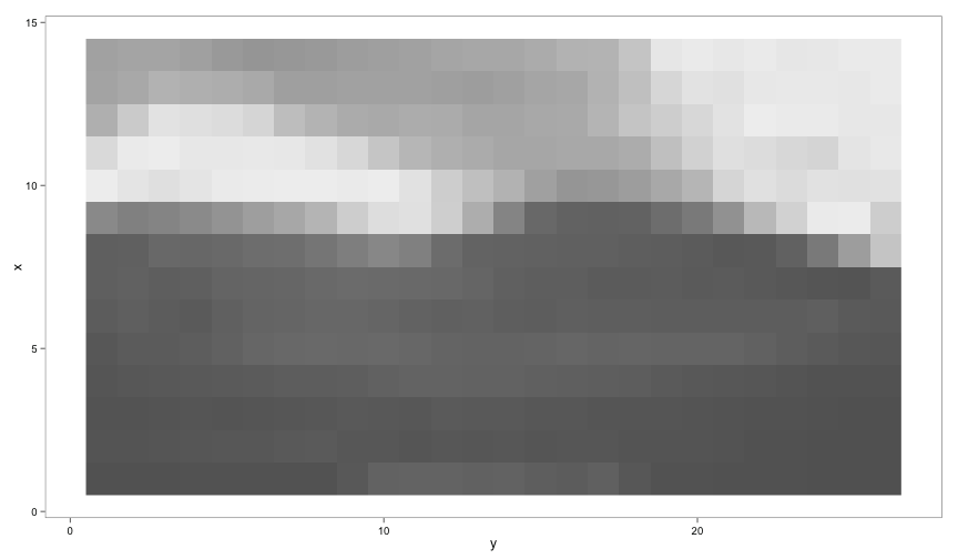
plot of chunk unnamed-chunk-11

# And now to predict if the image was taken during the day or at night.
# The predition is the probablity of the image having been taken during the day or at night.
predict(night_day_mod, get_sample(paste0("_Rmd/training_set/example/",file_to_test)))
##            day      night
## [1,] 0.9889661 0.01103407

Putting it all together

This section will outline how to use the models developed earlier to extract the images from multiple videos. The code extracts the images, classifies them, removes the unwanted images and stitches the images together using the desired frame rate.

# Create some directories to store the extracted image from.
# Move across to the folder with the time lapse videos
setwd("~/Desktop/timelapse/working")
# create a directory to store the images in
dir.create("images")
dir.create("finished")
# get the file names of the videos to process.
files_to_process <- dir(pattern=".AVI")
 
# The next part is a little long winded as it contains 
# a two nested for loops. Explanations can e found within the code below.
 
# Loop over the video files 
for(i in 1:length(files_to_process)){
  # Extract all of the image from the timelapse video and place them into 
  # the images directory
  system(paste0("ffmpeg -i ", 
                files_to_process[i]," -f image2 -q:v 1 images/tmp-%03d.jpeg"))
  # Get a list of the images which were just extracted
  images_to_process <- dir("images",pattern=".jpeg")
  # Create a list to store the processed dates in
  dates <- list()
  # Create a list to store the results of the day time or 
  # night time classification
  is_dark <- list()
  # Now loop over each image and classify them one by one.
  for(j in 1:length(images_to_process)){
    # Clip the image to get the timestamp part of the image
    datestamp <- extract_datestamp(paste0("images/",images_to_process[j]))
    # Extract the characters from the timestamp
    characters <- find_characters(datestamp, 14,14)
    # Predict each of the characters
    predicted_characters <- levels(timestamp_values)[max.col(
      predict(mod, characters))
      ]
    # Format the date and add it to the date list
    dates[[j]] <- ymd_hms(paste(as.character(predicted_characters), 
                                sep="", collapse = ""))
    # See if the photo was taken at night
    is_dark[[j]] <- max.col(predict(
      night_day_mod, 
      get_sample(paste0("images/",images_to_process[j]))))==2
    }
  # Now convert the dates and the dark list to vectors.
  dates <- do.call("c", dates)
  is_dark <- do.call("c", is_dark)
  dark_images <- !is_dark
  # Find which image was taken between 12 and 1 am.
  midnight_image <- hour(dates)==0
  # Create a vector to remove all night time images except the midnight image.
  remove_index <- (dark_images+midnight_image)==0
  # Remove the nigh time images.
  unlink(paste0("images/",images_to_process[remove_index]))
  
  # For the re-stitching back to a video ffmpeg requires the filenames to be incremental.
  # This next part renames all of the files in the correct order
  new_names <- paste0("tmp-", 
                      sprintf("%03d", 
                              1:length(images_to_process[!remove_index])), ".jpeg")
  for(j in 1:length(new_names)){
    system(paste0("mv images/",
                  images_to_process[!remove_index][j],
                  " finished/", new_names[j])) 
  }
  # And now put create the new video from the processed images.
  system(
    paste0("ffmpeg -f image2 -r 5 -i finished/tmp-%03d.jpeg -y -r 25 -q:v 1 final_",
           i,".mpg"))
}
 
# Now once the videos have been processed remove all the junk
unlink("finished", recursive = TRUE)
unlink("images", recursive = TRUE)
Introducting ggsnippets

In this post, I will introduce ggsnippets, which is a R package that contains a few helper functions for the infamous ggplot2 package. The package is currently on github and can be installed using the devtools package.

library(devtools)
install_github("johnDorian/ggsnippets")

The package has four functions:

  • facet_wrap_labeller
  • g_legend
  • rbind_ggplot_timeseries
  • grobsave

Facet wrap labeller

This function is heavily based on this answer on stackoverflow and provides the ability to change the labels of each facet.

For example the following plot has default names in the facets.

library(ggplot2)
library(gridExtra)
library(ggsnippets)
 
x_cars <- data.frame(cars, variable = sample(letters[1:5],
                                             50,
                                             replace = TRUE))
## Create the plot with facets
plt <- ggplot() + geom_point(aes(speed, dist), x_cars) +
  facet_wrap(~variable, ncol=1)
plt

plot of chunk unnamed-chunk-2

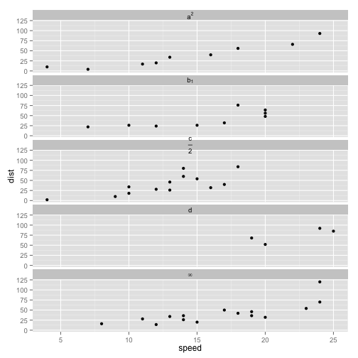
and now changing the labels

facet_wrap_labeller(plt, labels = c(expression(a^2),
                                    expression(b[1]),
                                    expression(frac(c,2)),
                                    "d",
                                    expression(infinity)))

plot of chunk unnamed-chunk-3

Extracting ggplot legends

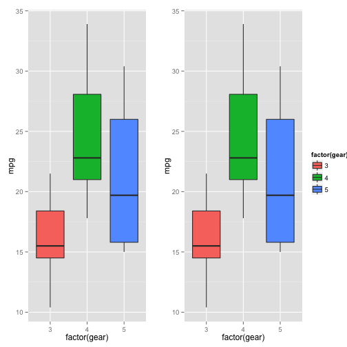
Sometimes it’s handy to be able to grab the legend from one ggplot and put it in another. This allows for the creation of a dummy plot to create a legend and use it in another plot. This function is stolen from this stackoverflow answer.

# Create a plot with a legend
plt <- ggplot() + 
  geom_boxplot(aes(factor(gear), mpg, fill=factor(gear)), mtcars)
# Extract the legend from the plot
plt_legend <- g_legend(plt)
# Create a new plot based on the orginal plot, but without a legend.
plt1 <- plt +  theme(legend.position="none")
# and create another plot without a legend.
plt2 <- plt +  theme(legend.position="none")
# Now stick the two plots together with the legend in a single row.
combined_plot <- arrangeGrob(plt1, plt2, plt_legend, nrow = 1, widths = c( 0.45, 0.45, 0.1))
combined_plot

plot of chunk unnamed-chunk-4

Combining multiple time series plots

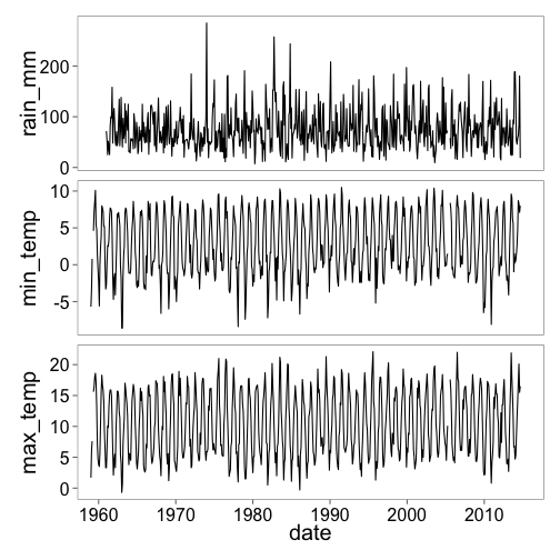
ggplot is a fantastic plotting package, but there are times when it doesn’t quite have the felxibility to plot the data in the desired way. This is espeically the case for time series data. The rbind_ggplot_timeseries function is designed to allow for the combination of several different ggplots with a date or datetime x axis. For example:

library(lubridate)
library(dplyr)
library(reshape2)
library(ggthemes)
data(breamardata)
breamardata$date <- ymd(paste(breamardata$year, breamardata$month, "1"))
 
# Create three plots without subsetting the data.
rain_plot <- ggplot() + geom_line(aes(date, rain_mm), breamardata) + theme_few(20)
min_temp_plot <- ggplot() + geom_line(aes(date, min_temp), breamardata) + theme_few(20)
max_temp_plot <- ggplot() + geom_line(aes(date, max_temp), breamardata) + theme_few(20)
 
# Plot all three together
combined_plot <- rbind_ggplot_timeseries(ggplot_list = 
                                           list(rain_plot,
                                                min_temp_plot,
                                                max_temp_plot
                                                ),
                                         limits = c(dmy("01011960", "31122014"))
                                         )
combined_plot

plot of chunk unnamed-chunk-5

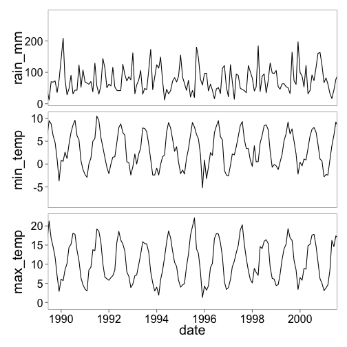
As the function allows for the limits of the x axis to be set, it is possible to zoom in to specfic moments of all plots. For example:

combined_plot <- rbind_ggplot_timeseries(ggplot_list = 
                                           list(rain_plot,
                                                min_temp_plot,
                                                max_temp_plot
                                                ),
                                         limits = c(dmy("01011990", "31122000"))
                                         )
combined_plot

plot of chunk unnamed-chunk-6

Finally…

The last function grobsave provides a modified version of ggplot2::ggsave which allows for the saving of grob style objects. This can be used to save the plots produced using the rbind_ggplot_timeseries function or the combination of plots outlined earlier where two plots and one legend were combined using the arrangeGrob function.

Currently the package only contains the four functions listed above. Howvever, I am considering adding an additional function which should help with plotting two time series on one plot using two y-axis.

Creating a Spatial Stream Network with GRASS GIS. Part I

Recently, I wanted to use the SSN R package to predict along a stream network. To do this you need to set up the GIS files using the ArcGIS plugins here. I don’t have access to ArcGIS (and I don’t want it) because I only have access to ubuntu and OS X. This is why I decided to develop several GRASS GIS addons to provide the capability to create ssn objects to be used in R. This post will outline the first few steps used in delineating catchments in R and I will follow this post up with the addons later on.

I am going to outline how to create a ssn object in GRASS using the workshop data which can be found here: ssn-short-course.

Step 1: Creating the project

  1. Create a new Project location Project location window
  2. Give it a name Name of new Project
  3. You now need to set the project, resolution and bounds of your project. The easiest way to do this is to select the third option and choose the dem file datasets/gisdata/dem/w001001.adf. Project settings
  4. You will now be given the option to import the file into the project. Select No - will we do this later
  5. Now you will be given the option to create a working directory. From my understanding this option exists to provide flexibility for multiple users. I prefer to use the term “working”, but this doesn’t matter.
  6. Now you can start the grass session.

Step 2: Importing the maps

Below I will provide the list of commands which can be used directly in the command console within GRASS. You don’t need to use the commands as the GUI does have list most of the commands I will use. You can also use the command console to open an additional window for each grass command. For example you can type: r.in.gdal and press enter. This will open the import window. Import raster window

Import the DEM map (the ‘e’ flag tells GRASS to set the bounds and resolution to the DEM map)

bash r.in.gdal input=/Users/jasonlessels/work/Projects/ssn-short-course/datasets/gisdata/dem/w001001.adf output=dem -e

You can display the DEM map Location elevation

To import the developed land classified map

bash r.in.gdal input=/Users/jasonlessels/work/Projects/ssn-short-course/datasets/gisdata/developd/w001001.adf output=developed

Import the site location vector layer

bash v.in.ogr input=/Users/jasonlessels/work/Projects/ssn-short-course/datasets/gisdata/sub_sites.shp layer=sub_sites output=sites

Import the streams

bash v.in.ogr input=/Users/jasonlessels/work/Projects/ssn-short-course/datasets/gisdata/streams.shp layer=streams output=streams

Step 3: Filling in sinks and burning in streams.

Now I will outline how you can correct for sinks in the DEM raster, and if you want to, burn in the streams. Burning in the streams is handy if you have access to data with the locations of real streams.

Convert the streams (vector) to a raster

bash v.to.rast --overwrite input=streams@working type=line output=gov_streams use=cat

Subtract 10 m elevation from the DEM where streams lie.

bash r.mapcalc expression='dem_burn = if(!isnull(gov_streams), dem-10, dem)'

Fill the DEM and create a direction map.

bash r.fill.dir input=dem_burn@working output=dem_filled direction=fill_direction

Create accumulation map

bash r.watershed elevation=dem_filled threshold=250000 accumulation=accum

Extract streams using the r.streams modules.

bash r.stream.extract elevation=dem_filled accumulation=accum threshold=2500 stream_rast=stream_rast stream_vect=stream_vect direction=direction

Install the additional r.stream* addons.

bash g.extension extension=r.stream.order operation=add g.extension extension=r.stream.snap operation=add g.extension extension=r.stream.distance operation=add

Obtain the stream order

bash r.stream.order stream_rast=stream_rast direction=direction elevation=dem_filled accumulation=accum stream_vect=stream_order

The r.stream.order function add several additional columns with data. The names get truncated when they are exported as a shape file. The next few lines truncates the names now.

bash v.db.renamecolumn map=stream_order column='next_stream, nxt_str' v.db.renamecolumn map=stream_order column='scheidegger, scheide' v.db.renamecolumn map=stream_order column='source_elev, src_elev' v.db.renamecolumn map=stream_order column='outlet_elev, olt_elev' v.db.renamecolumn map=stream_order column='stream, rid' v.db.renamecolumn map=stream_order column='out_dist, upDist'

Snap the points to the streams using the r.stream.snap function. This will create a new vector layer. The radius is set to 10 m and the function will move the sites to the streams if the points are within 10 meters of a stream. This function also provides the ability to see if the points were moved or not.

bash r.stream.snap input=sites output=snap_sites stream_rast=stream_rast accumulation=accum radius=10

Add an attribute table to the snap_sites vector (Seems to be a bug)

bash v.db.addtable map=snap_sites table=snap_sites

Join the table with the sites table - this can take a minute or so.

bash v.db.join map=snap_sites column=cat otable=sites ocolumn=cat

Step 4. Site distance ratio

Now estimate the distance ratio for each. This is done by getting the distance to the end of each node for every cell and dividing it by the length of each edge.

Get the distance to the end of the entire network.

bash r.stream.distance -o stream_rast=stream_rast direction=direction elevation=dem_filled method=downstream distance=distance

Get the length of each edge and convert it to a raster.

bash v.to.rast input=stream_order type=line output=edge_length use=attr attrcolumn=length v.to.rast input=stream_order type=line output=upDist use=attr attrcolumn=upDist

Calculate the distance ratio for each edge.

bash r.mapcalc expression='distance_ratio=if(!isnull( edge_length),(distance - (upDist-edge_length))/edge_length , null())'

Calculate point upDist - this should be the same as upDist, but do it again anyway.

bash r.mapcalc expression='point_dist=if(!isnull( edge_length),(distance_ratio*edge_length)+(upDist-edge_length) , null())'

Step 5. Update the sites vector

Firstly, new columns have to be added to the snap_sites vector

bash v.db.addcolumn map=snap_sites columns='rid INT, netID INT, pid INT, locID INT, ratio double precision, NEAR_X double precision, NEAR_Y double precision, upDist double precision, elev double precision'

Now use the v.what.vect function to get the corresponding values from the raster maps.

bash v.what.vect map=snap_sites column=rid qmap=stream_order qcolumn=rid v.what.vect map=snap_sites column=netID qmap=stream_order qcolumn=netID v.what.rast map=snap_sites raster=distance_ratio column=ratio v.what.rast map=snap_sites raster=point_dist column=upDist v.what.rast map=snap_sites raster=dem column=elev

Create a prediction id column based on the

bash v.db.update map=snap_sites layer=1 column=pid qcolumn=cat v.db.update map=snap_sites layer=1 column=locID qcolumn=cat

Add x and y coordinates to the snap_sites vector using the v.to.db function.

bash v.to.db map=snap_sites option=coor col=NEAR_X,NEAR_Y

Step 6. Create a prediction grid

Create the predictions points using the v.to.points function. This will create a point every 1500 m along the stream

bash v.to.points input=stream_order type=line output=pred_pts dmax=1500

The vector created above has two tables - the table of stream_order and a new table for all the new points, named;

  1. table 1 = pred_pts_1
  2. table 2 = pred_pts_2

The next step is to use the lcat (which is the same as the rid) to merge the tables together.

bash v.db.join map=pred_pts layer=2 column=lcat otable=pred_pts_1 ocolumn=rid scolumns=rid,length,upDist,netID

Calculate the up stream distance for each point using the along and upDist columns. The v.to.points function added an along column, which is the distance from the node of every edge.

bash v.db.update pred_pts col=upDist qcol="along+(upDist-length)" layer=2

Add new columns for the prediction points

bash v.db.addcolumn map=pred_pts layer=2 columns='pid INT, locID INT, ratio double precision, NEAR_X double precision, NEAR_Y double precision, elev double precision'

Now update the table

bash v.db.update pred_pts col=locID qcol="pid" layer=2 v.db.update pred_pts col=ratio qcol="round(along/length, 2)" layer=2 v.to.db map=pred_pts layer=2 option=coor col=NEAR_X,NEAR_Y v.what.rast map=pred_pts raster=lidar_dem column=elev layer=2

Use the v.db.univar function to find the maximum pid value.

bash v.db.univar -g map=snap_sites column=pid

Alternativitly, you can assign the values to the shell window to be used latter.

bash eval $(v.db.univar -g map=snap_sites column=pid)

This will give you all the stats from the map in the bash session and you can access them like:

bash echo $max

Now you can update the value of the pid columns which will be greater than all the values in the observations to make sure there are no duplicated pid values

bash v.db.update pred_pts col=pid qcol="$max+cat" layer=2

Step 7. Getting contributing area and covariate stats

to be continued…