Introducting ggsnippets
02 Apr 2015In this post, I will introduce ggsnippets, which is a R package that contains a few helper functions for the infamous ggplot2 package. The package is currently on github and can be installed using the devtools package.
library(devtools)
install_github("johnDorian/ggsnippets")
The package has four functions:
facet_wrap_labellerg_legendrbind_ggplot_timeseriesgrobsave
Facet wrap labeller
This function is heavily based on this answer on stackoverflow and provides the ability to change the labels of each facet.
For example the following plot has default names in the facets.
library(ggplot2)
library(gridExtra)
library(ggsnippets)

x_cars <- data.frame(cars, variable = sample(letters[1:5],
                                             50,
                                             replace = TRUE))
## Create the plot with facets
plt <- ggplot() + geom_point(aes(speed, dist), x_cars) +
  facet_wrap(~variable, ncol=1)
plt
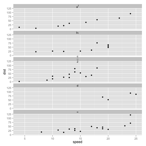
and now changing the labels
facet_wrap_labeller(plt, labels = c(expression(a^2),
                                    expression(b[1]),
                                    expression(frac(c,2)),
                                    "d",
                                    expression(infinity)))
Extracting ggplot legends
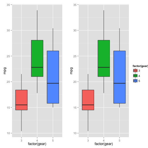
Sometimes it’s handy to be able to grab the legend from one ggplot and put it in another. This allows for the creation of a dummy plot to create a legend and use it in another plot. This function is stolen from this stackoverflow answer.
# Create a plot with a legend
plt <- ggplot() +
  geom_boxplot(aes(factor(gear), mpg, fill=factor(gear)), mtcars)
# Extract the legend from the plot
plt_legend <- g_legend(plt)
# Create a new plot based on the orginal plot, but without a legend.
plt1 <- plt +  theme(legend.position="none")
# and create another plot without a legend.
plt2 <- plt +  theme(legend.position="none")
# Now stick the two plots together with the legend in a single row.
combined_plot <- arrangeGrob(plt1, plt2, plt_legend, nrow = 1, widths = c( 0.45, 0.45, 0.1))
combined_plot
Combining multiple time series plots
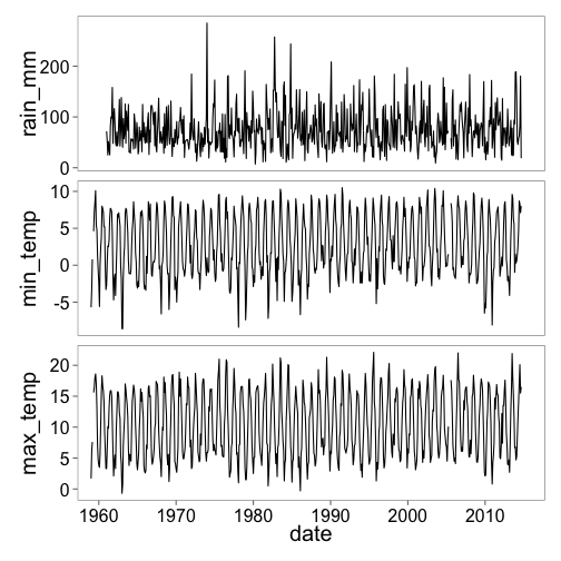
ggplot is a fantastic plotting package, but there are times when it doesn’t quite have the felxibility to plot the data in the desired way. This is espeically the case for time series data. The rbind_ggplot_timeseries function is designed to allow for the combination of several different ggplots with a date or datetime x axis. For example:
library(lubridate)
library(dplyr)
library(reshape2)
library(ggthemes)
data(breamardata)
breamardata$date <- ymd(paste(breamardata$year, breamardata$month, "1"))

# Create three plots without subsetting the data.
rain_plot <- ggplot() + geom_line(aes(date, rain_mm), breamardata) + theme_few(20)
min_temp_plot <- ggplot() + geom_line(aes(date, min_temp), breamardata) + theme_few(20)
max_temp_plot <- ggplot() + geom_line(aes(date, max_temp), breamardata) + theme_few(20)

# Plot all three together
combined_plot <- rbind_ggplot_timeseries(ggplot_list =
                                           list(rain_plot,
                                                min_temp_plot,
                                                max_temp_plot
                                                ),
                                         limits = c(dmy("01011960", "31122014"))
                                         )
combined_plot
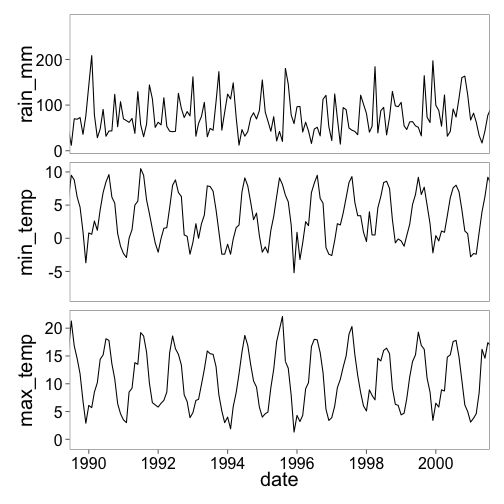
As the function allows for the limits of the x axis to be set, it is possible to zoom in to specfic moments of all plots. For example:
combined_plot <- rbind_ggplot_timeseries(ggplot_list =
                                           list(rain_plot,
                                                min_temp_plot,
                                                max_temp_plot
                                                ),
                                         limits = c(dmy("01011990", "31122000"))
                                         )
combined_plot
Finally…
The last function grobsave provides a modified version of ggplot2::ggsave which allows for the saving of grob style objects. This can be used to save the plots produced using the rbind_ggplot_timeseries function or the combination of plots outlined earlier where two plots and one legend were combined using the arrangeGrob function.
Currently the package only contains the four functions listed above. Howvever, I am considering adding an additional function which should help with plotting two time series on one plot using two y-axis.